Python Tutorial 2: Hidden Markov Models
(C) 2016-2019 by Damir Cavar <dcavar@iu.edu>
Version: 1.1, September 2019
Download: This and various other Jupyter notebooks are available from my GitHub repo.
This is a tutorial about developing simple Part-of-Speech taggers using Python 3.x, the NLTK (Bird et al., 2009), and a Hidden Markov Model (HMM).
This tutorial was developed as part of the course material for the course Advanced Natural Language Processing in the Computational Linguistics Program of the Department of Linguistics at Indiana University.
Hidden Markov Models
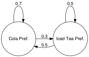
Given a Hidden Markov Model (HMM), we want to calculate the probability of a state at a certain time, given some evidence via some sequence of emissions. Let us assume the following HMM as described in Chapter 9.2 of Manning and Schütze (1999):
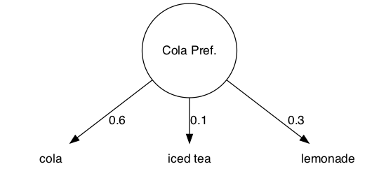
The emission probabilities for cola, iced tea, and lemonade when the machine is in state Cola Pref. are:
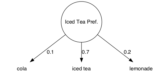
When the machine is in the Iced Tea Pref. state, the emission probabilities for the three different beverages are:
We can describe the machine using state and emission matrices. The state matrix would be:
| Cola Pref. | Iced Tea Pref. | |
|---|---|---|
| Cola Pref. | 0.7 | 0.3 |
| Iced Tea Pref. | 0.5 | 0.5 |
The emission matrix is:
| cola | iced tea | lemonade | |
|---|---|---|---|
| Cola Pref. | 0.6 | 0.1 | 0.3 |
| Iced Tea Pref. | 0.1 | 0.7 | 0.2 |
We can describe the probability that the soda machine starts in a particular state, using an initial probability matrix. If we want to state that the machine always starts in the Cola Pref. state, we specify the following initial probability matrix that assignes a 0 probability to the state Iced Tea Pref. as a start state:
| State | Prob. |
|---|---|
| Cola Pref. | 1.0 |
| Iced Tea Pref. | 0.0 |
We can represent these matrices using Python numpy data structures. If you are using the Anaconda release, the numpy module should be already part of your installation. To import the numpy module, use the following command:
import numpy
The state matrix could be coded in the following way:
stateMatrix = numpy.matrix("0.7 0.3; 0.5 0.5")
You can inspect the stateMatrix content:
stateMatrix
The emission matrix can be coded in the same way:
emissionMatrix = numpy.matrix("0.6 0.1 0.3; 0.1 0.7 0.2")
You can inspect the emissionMatrix content:
emissionMatrix
And finally we can encode the initial probability matrix as:
initialMatrix = numpy.matrix("1 0")
We can inspect it using:
initialMatrix
Given some observation of outputs from the crazy soda machine, we want to calculate the most likely sequence of hidden states. Assume that we observe the following:
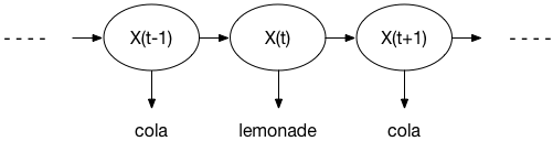
We are asking for the most likely sequence of states $X(t-1),\ X(t),\ X(t+1)$ for the given observation that the machine is delivering the products cola lemonade cola in that particular sequence. We can calculate the probability by assuming that we start in the Cola Pref. state, as expressed by the initial probability matrix. That is, computing the paths or transitions starting from any other start state would have a $0$ probability and are thus irrelevant. For only two observations cola lemonade there are 4 possible paths through the HMM above, this is: Cola Pref. and Iced Tea Pref., Cola Pref. and Cola Pref., Iced Tea Pref. and Iced Tea Pref., Iced Tea Pref. and Cola Pref.. For three observations cola lemonade cola we have 8 paths with a probability larger than $0$ through our HMM. To compute the probability for a certain sequence to be emitted by our HMM taking one path, we would multiply the products of the state transition probability and the output emission probability at every time point for the observation. We would sum up the products of all these probabilities for all possible paths through our HMM to compute the general probability of our observation.
In the Cola Pref. state we would have a probability to transit to the Cola Pref. state of $P(Cola\ Pref.\ |\ Cola\ Pref.) = 0.7$ and the likelihood to emit a cola is $P(cola) = 0.6$. That is, for the first step we would have to multiply:
We will have to multiply this first step result now with the probabilities of the next steps for a given path. Let us assume that our machine decides to transit to the Iced Tea Pref. state with $P(Iced\ Tea\ Pref.\ |\ Cola\ Pref.) = 0.3$. The emission probability for lemonade would then be $P(lemonade\ |\ Iced\ Tea\ Pref.) = 0.2$. The probability for this sub-path so far given the observation cola lemonade would thus be:
$$0.7 * 0.6 * 0.3 * 0.2 = 0.0252$$
Let us assume that the next step that the machine takes is a step back to the $Cola\ Pref.$ state. The likelihood of the transition is $P(Cola\ Pref.\ |\ Iced\ Tea\ Pref.) = 0.5$. The likelihood to emit cola from the target state is $P(cola\ |\ Cola\ Pref.) = 0.6$. The likelihood of observing the emissions (cola, lemonade, cola) in that particular sequence when starting in the Cola Pref. state and when taking a path through the states (Cola Pref., Iced Tea Pref., Cola Pref.) is thus $0.7 * 0.6 * 0.3 * 0.2 * 0.5 * 0.6$. Now we would have to sum up this probability with the respective probabilities for all the other possible paths.
Decoding
The Forward Algorithm
For more detailed introductions and overviews see for example Jurafsky and Klein (2014, draft) Chapter 8, or Wikipedia.
If we would want to calculate the probability of a specific observation like cola lemonade cola for a given HMM, we would need to calculate the probability of all possible paths through the HMM and sum those up in the end. To calculate the probability of all possible paths, we would
This equation is computationally demanding. It would require $O(2Tn^T)$ calculations. To reduce the computational effort, the Forward Algorithm makes use of a dynamic programming strategy to store all intermediate results in a trellis or matrix. We can display the
The Forward-Backward Algorithm
Coming soon
Viterbi Algorithm
Coming soon
Training an HMM tagger using NLTK
We will use the Penn treebank corpus in the NLTK data to train the HMM tagger. To import the treebank use the following code:
from nltk.corpus import treebank
We need to import the HMM module as well, using the following code:
from nltk.tag import hmm
We can instantiate a HMM-Trainer object and assign it to a trainer variable using:
trainer = hmm.HiddenMarkovModelTrainer()
As you can recall from the Part-of-Speech tagging tutorial, the function brown.tagged_sents() returns a list sentences which are lists of tuples of token-tag pairs. The following function returns the first two tagged sentences from the Brown corpus:
treebank.tagged_sents()[:2]
The NLTK HMM-module offers supervised and unsupervised training methods. Here we train an HMM using a supervised (or Maximum Likelihood Estimate) method and the Brown corpus:
tagger = trainer.train_supervised(treebank.tagged_sents())
We can print out some information about the resulting tagger:
tagger
The tagger expects a list of tokens as a parameter. We can import the NLTK word_tokenize module to tokenize some input sentence and tag it:
from nltk import word_tokenize
The function word_tokenize takes a string as parameter and returns a list of tokens:
word_tokenize("Today is a good day.")
We can tag an input sentence by providing the output from the tokenizer as the input parameter to the tag method of the tagger-object:
tagger.tag(word_tokenize("Today is a good day."))
References
Bird, Steven, Ewan Klein, Edward Loper (2009) Natural Language Processing with Python: Analyzing Text with the Natural Language Toolkit. O'Reilly Media.
Jurafsky, Daniel, James H. Martin (2014) Speech and Language Processing. Online draft of September 1, 2014.
Manning, Chris and Hinrich Schütze (1999) Foundations of Statistical Natural Language Processing, MIT Press. Cambridge, MA.
(C) 2016-2019 by Damir Cavar <dcavar@iu.edu>